The preparations will be shorter, since I am just revising core 3D CV concepts and perhaps some papers
The first chapter consists of Camera Models, Single-View Metrology and Epipolar Geometry. For the core concepts I am following the Stanford Course: CS231A: Computer Vision, From 3D Reconstruction to Recognition
Stay tuned for the next lessons!
We start with the camera, which is the system that lets us record the real 3D world. Pay attention to core concepts. Without having these fundamental, it will be harder to follow the more advanced papers!
There are 2 ways to model the camera that are the most popular: Pinhole Cameras and Lens Cameras.
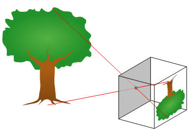
Pinhole cameras are designed by putting a wall at least as tall as the 3D object itself (and as large as the 3D object horizontally, while obviously being perpendicular(loosely defined, the definition of perpendicularity in these cases)) , and by putting a small hole in the wall, just like the figure above.
We want to emit light from every point of the 3D object towards the wall, such that the wall stops the light and the hole lets it continue to the other side,and by observing one can see that, at the other side, we get an upside-down image in what we call the image plane or retinal plane.
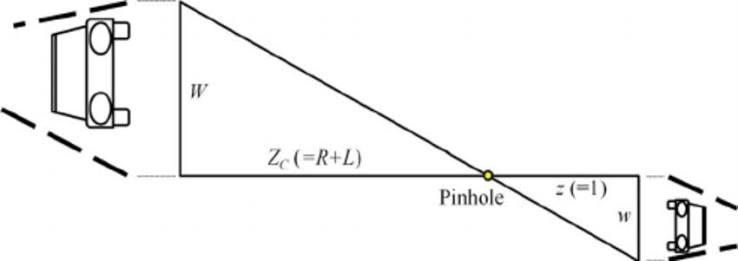
Notation: \(O\) is the coordinate of the hole/aperture, called origin. The distance between the origin and the image plane is focal length \(f\). Sometimes, for visualization reasons, the retinal plane is placed between \(O\) and the 3D object at a distance \(f\) from \(O\). In this case, it is called the virtual image or virtual retinal plane. You can experiment to what happens when you change any variable.
Now that we defined the pinhole camera, how do we actually use it? Let \(P = \begin{bmatrix} x & y & z \end{bmatrix}^T\) be the 3D point on the object that is visible from the aperture. We want to map \(P\) to the image plane \(\Pi'\), resulting in \(P' = \begin{bmatrix} x & y \end{bmatrix}^T\). The term projection is just representing the 3D object onto a 2D flat surface/plane.
We now define a new coordinate system \(\begin{bmatrix} i & j & k \end{bmatrix}\) with origin at the hole \(O\). We define the axis \(k\) as perpendicular to the image plane, with the positive numbers going towards the image. This coordinate system is often known as the camera reference system or camera coordinate system (these 2 terms are ambiguous, just memorize them in my opinion). The line defined by \(C'\) and \(O\) is called the optical axis of the camera system (\(C'\) is the projection of the pinhole onto the image plane).
Now, since \(P'\) depends on \(P\), if we derive the relationship between the 2 points \(P\) and \(P'\), we can understand the 3D world and how it imprints itself on the image made bby the camera.
This section is the part I had a hard time thinking about, but then I heard an explanation and it just made sense: observe the triangles \(P'C'O\) and \(P\,O\,(0, 0, z)\). these have similar angles and by law of similarity of triangles, this holds: \[ \frac{x'}{f} = \frac{x}{z} \;\Rightarrow\; x' = \frac{f\,x}{z} \] also for the \(y\) axis: \[ \frac{y'}{f} = \frac{y}{z} \;\Rightarrow\; y' = \frac{f\,y}{z} \] hence \[ P' = \begin{bmatrix} x' \\ y' \end{bmatrix} = \begin{bmatrix} f\,\frac{x}{z} \\[4pt] f\,\frac{y}{z} \end{bmatrix} \]
The interactive visualization does not show that while shortenin the aperture size makes it crispier, it also makes it darker. Less light coming in! Can we make a camera that takes bright AND crispy images? Yes: Lens cameras.
Lenses are devices that can concentrate/focus or disperse light.
If we replace the pinhole with a properly placed and sized lens, then we have this nice property: all rays of light that the 3D point P emits, are refracted (moved) by the lens such that they converge to a single point P' in the 2D image plane. Therefore, the problem of the majority of the light rays blocked due to a small aperture is removed. However, this property does not hold for all 3D points, but only for some specific point P . Take another point Q which is closer or further from the image plane than P . The corresponding projection into the image will be blurred or out of focus. Therefore, lenses have a specific distance for which objects are “in focus”.
Another advantageous property: Camera lenses have another interesting property: they focus all light rays traveling parallel to the optical axis to one point known as the focal point
The distance between the focal point and the center of the lens is commonly referred to as the focal length f (similar to the pinhole, but now we have an additional length). Furthermore, light rays passing through the center of the lens are not deviated. We thus can arrive at a similar construction to the pinhole model that relates a point P in 3D space with its corresponding point P' in the image plane.
A lens bends every ray from a point so they meet again at \(z_i\), given by \(\frac{1}{f} = \frac{1}{z_o} + \frac{1}{z_i}\). Only if the sensor sits exactly there is the image sharp; elsewhere the point spreads into a blur circle. Shrink the aperture to see the blur shrink (larger depth of field).
Furthermore, light rays passing through the center of the lens are not deviated. We thus can arrive at a similar construction to the pinhole model that relates a point \(P\) in 3D space with its corresponding point \(P'\) in the image plane: \[ P' = \begin{bmatrix} x' \\ y' \end{bmatrix} = \begin{bmatrix} z'\,\frac{x}{z} \\[4pt] z'\,\frac{y}{z} \end{bmatrix} \] The derivation for this model is not important, and too advanced to be worth learning it at this stage.
For both pinhole and lens cameras, the projection from the 3D world to the image plane does not correspond to what one sees in actual digital images, and this is for specific reasons. First, points in the digital images are, in general, in a different reference system than those in the image plane (light hitting a camera's sensor and the digital array of pixels stored in computer memory). Second, similarly, digital images are divided into discrete pixels, whereas points in the image plane are continuous. Third, the physical sensors from the camera can introduce non-linearity such as distortion to the mapping. (In a perfectly linear system, if you take a photo of a straight line, the math guarantees it will map to perfectly straight pixels. Matrix multiplication can only scale, rotate, or shift the image,it cannot bend it.) Hence we need to a number of additional transformations that allow us to map any point from the 3D world to pixel coordinates.
The camera matrix model is a way of describing parameters that affect how a 3D point \(P\) is mapped to \(P'\). These parameters are put into a matrix, hence the name. Let's talk about those parameters.
The first parameters, \(c_x\) and \(c_y\), show the difference in translation between the digital image and the image plane (perhaps confusing wording, remember that the digital image is made of pixels). Image plane coordinates have their origin at \(C'\), the image center, where the \(k\) axis makes contact with the image plane. Digital images instead usually have their origin in the lower-left corner of the image . So the same point has different coordinates in the two systems, and the difference is just a shift by the vector \(\begin{bmatrix} c_x & c_y \end{bmatrix}^T\). We add it to the mapping we found before: \[ P' = \begin{bmatrix} x' \\ y' \end{bmatrix} = \begin{bmatrix} f\,\frac{x}{z} + c_x \\[4pt] f\,\frac{y}{z} + c_y \end{bmatrix} \]
The second thing to work with is the units. Points in the digital image are expressed in pixels, while points in the image plane are expressed in physical units (centimeters, for example). So we need 2 new parameters, \(k\) and \(l\), with units \(\frac{\text{pixels}}{\text{cm}}\), that tell us how many pixels fit in one unit of length along each of the two axes. We define k and l differently since the pixels may not be square. If \(k = l\) we say that the camera has square pixels. The mapping becomes: \[ P' = \begin{bmatrix} x' \\ y' \end{bmatrix} = \begin{bmatrix} f\,k\,\frac{x}{z} + c_x \\[4pt] f\,l\,\frac{y}{z} + c_y \end{bmatrix} = \begin{bmatrix} \alpha\,\frac{x}{z} + c_x \\[4pt] \beta\,\frac{y}{z} + c_y \end{bmatrix} \] where \(\alpha = f\,k\) and \(\beta = f\,l\).
(interlude to homogeneous coordinates) Now, next problem: we would love to write this projection as a matrix times a vector, \(P' = M P\), because matrices are easy to chain together and all the later derivations rely on that. But a matrix-vector product can only represent a linear transformation, and ours is not linear: we are dividing by \(z\), which is one of the inputs. No \(2 \times 3\) matrix multiplied by \(\begin{bmatrix} x & y & z \end{bmatrix}^T\) can produce a \(\frac{x}{z}\). So, can we still write it as a matrix-vector product? Yes, with homogeneous coordinates.
The simple trick these people have found is to change the coordinate system by adding one extra coordinate. A 2D point \(P' = (x', y')\) becomes \((x', y', 1)\), and a 3D point \(P = (x, y, z)\) becomes \((x, y, z, 1)\). This augmented space is called the homogeneous coordinate system.
The rules to go back and forth are simple:
The second rule is the whole point of why we do this. It means that a homogeneous vector and any multiple of it are the same Euclidean point: \((2, 4, 2)\) and \((1, 2, 1)\) both represent the 2D point \((1, 2)\). A vector is equal to its Euclidean version only when the last coordinate is 1.
See what this gives us? The division that was bothering us is now hidden inside the conversion back to Euclidean coordinates. If we manage to put \(z\) in the last coordinate of the output, the division by \(z\) happens "for free" at the end, and everything before it can be linear. Multiply our mapping by \(z\) and this is exactly what we get: \[ P'_h = \begin{bmatrix} \alpha x + c_x z \\ \beta y + c_y z \\ z \end{bmatrix} = \begin{bmatrix} \alpha & 0 & c_x & 0 \\ 0 & \beta & c_y & 0 \\ 0 & 0 & 1 & 0 \end{bmatrix} \begin{bmatrix} x \\ y \\ z \\ 1 \end{bmatrix} \] Check it yourself: dividing the first two entries of \(P'_h\) by the third one gives back \(\alpha\frac{x}{z} + c_x\) and \(\beta\frac{y}{z} + c_y\), the same mapping as before. Every entry of \(P'_h\) is now a linear combination of \(x, y, z\), so the projection is a plain matrix-vector product.
A quick example with numbers. Take \(\alpha = \beta = 800\), \(c_x = 320\), \(c_y = 240\) and the 3D point \(P = (0.5,\, 0.25,\, 2)\): \[ \begin{bmatrix} 800 & 0 & 320 & 0 \\ 0 & 800 & 240 & 0 \\ 0 & 0 & 1 & 0 \end{bmatrix} \begin{bmatrix} 0.5 \\ 0.25 \\ 2 \\ 1 \end{bmatrix} = \begin{bmatrix} 1040 \\ 680 \\ 2 \end{bmatrix} \;\rightarrow\; \left(\frac{1040}{2}, \frac{680}{2}\right) = (520,\, 340) \] So \(P\) lands on the pixel \((520, 340)\). If you move the point twice as far, \(P = (0.5,\, 0.25,\, 4)\), you get \((420, 290)\): closer to the center \((320, 240)\), as you would expect from something further away.
From now on we assume everything is in homogeneous coordinates and drop the \(h\) index. The relationship between a 3D point and its image coordinates is: \[ P' = \begin{bmatrix} \alpha & 0 & c_x & 0 \\ 0 & \beta & c_y & 0 \\ 0 & 0 & 1 & 0 \end{bmatrix} P = M P \] Notice that the last column of \(M\) is all zeros, so it does nothing. We can split it off: \[ P' = M P = \begin{bmatrix} \alpha & 0 & c_x \\ 0 & \beta & c_y \\ 0 & 0 & 1 \end{bmatrix} \begin{bmatrix} I & 0 \end{bmatrix} P = K \begin{bmatrix} I & 0 \end{bmatrix} P \] where \(I\) is the \(3 \times 3\) identity and \(0\) is a column of zeros. The matrix \(K\) is the camera matrix.
Two things are still missing from \(K\): skewness and distortion.
An image is skewed when the two axes of the sensor are not exactly perpendicular, so the angle \(\theta\) between them is slightly more or less than 90 degrees. Think of the pixels as tiny parallelograms instead of rectangles. Most cameras have zero skew, but manufacturing errors in the sensor can introduce a bit of it. The derivation is not worth going through at this stage, the result is: \[ K = \begin{bmatrix} \alpha & -\alpha \cot\theta & c_x \\[2pt] 0 & \frac{\beta}{\sin\theta} & c_y \\[2pt] 0 & 0 & 1 \end{bmatrix} \] Sanity check: with \(\theta = 90°\) we have \(\cot\theta = 0\) and \(\sin\theta = 1\), and we are back to the \(K\) from before.
Distortion is ignored for now (matrix multiplication cannot bend lines, remember?), so it does not appear in \(K\). This means that \(K\) has 5 degrees of freedom: 2 for the focal length (\(\alpha, \beta\)), 2 for the offset (\(c_x, c_y\)) and 1 for the skew (\(\theta\)). These are called the intrinsic parameters, because they are properties of the camera itself, of how it was built. They do not change if you pick the camera up and move it somewhere else.
Until now the point \(P\) was expressed in the camera reference system, the one with the origin at the pinhole \(O\). But usually the 3D world is described in some other coordinate system: the corner of a room, the center of an object, a GPS frame. We call it the world reference system. So before projecting, we need one more transformation that takes a point from the world reference system to the camera reference system.
This transformation is a rotation matrix \(R\) (\(3 \times 3\)) followed by a translation vector \(T\) (\(3 \times 1\)). In Euclidean coordinates it would be \(P = R\,P_w + T\); in homogeneous coordinates the sum disappears and it becomes a single matrix: \[ P = \begin{bmatrix} R & T \\ 0 & 1 \end{bmatrix} P_w \] \(P_w\) is the point in the world reference system. This is just another nice thing about homogeneous coordinates: a translation, which is not linear in Euclidean coordinates, becomes a matrix multiplication.
Now we substitute this into \(P' = K \begin{bmatrix} I & 0 \end{bmatrix} P\): \[ P' = K \begin{bmatrix} I & 0 \end{bmatrix} \begin{bmatrix} R & T \\ 0 & 1 \end{bmatrix} P_w = K \begin{bmatrix} R & T \end{bmatrix} P_w = M P_w \] The \(\begin{bmatrix} I & 0 \end{bmatrix}\) just throws away the last row \(\begin{bmatrix} 0 & 1 \end{bmatrix}\), leaving \(\begin{bmatrix} R & T \end{bmatrix}\).
\(R\) and \(T\) are called the extrinsic parameters, because they are external to the camera: they only say where the camera is and where it is looking.
To sum up, the full projection matrix \(M = K \begin{bmatrix} R & T \end{bmatrix}\) is a \(3 \times 4\) matrix that takes a 3D point in any world reference system all the way to pixel coordinates. It has 11 degrees of freedom:
It also makes sense from another angle: \(M\) has 12 entries, but in homogeneous coordinates \(M\) and any multiple of it give the same image point, so one entry is used for the scale. 12 − 1 = 11.
This argument had me thinking for a bit. But please try to concentrate and follow me.
Camera calibration is needed when we are trying to understand the transformation from the 3D world into the digital image, but we do not have access to intrinsic parameters, such as focal length, offset, skewness. What we do have is access to the photos it takes. How do we go on and find the instrinsic AND extrinsic parameters? This problem is called the Camera Calibration Problem
Obviously, now what we must do is solving for the intrinsic camera matrix K and the extrinsic parameters \(R, T\) from \(M P_w\)
The description of this problem is done with a Calibration Rig.
The calibration rig consists of a discrete mapping from the 3D world to the 2D image. The 3D world is usually a checkerboard, with known dimensions. Furthermore, the rig defines our world reference frame with origin \(O_w\) and axes \(i_w, j_w, k_w\). From the rig's known pattern, we have known points in the world reference frame \(P_1, ..., P_n\). Finding these points in the image we take from the camera gives corresponding points in the image \(p_1, ..., p_n\).
If one wants to understand this, he or she needs to think about the following linear system which we set up, with n correspondences such that for each correspondence \(P_i, p_i\) and camera matrix \(M\) whose rows are \(m_1, m_2, m_3\): \[ p_i = \begin{bmatrix} u_i \\ v_i \end{bmatrix} = MP_i = \begin{bmatrix} \frac{m_1P_i}{m_3P_i} \\[4pt] \frac{m_2P_i}{m_3P_i}\end{bmatrix} \] Think about what the last part of the equation does, by dividing \(m_1P_i\) by \(m_3P_i\). Originally it was 3 rows, but for homogeneity, we divided every row by the last one, hence the \(_3P_i\)
Each correspondence gives us two equations and, consequently, two constraints for solving the unknown parameters contained in \(m\). From before, we know that the camera matrix has 11 unknown parameters. This means that we need at least 6 correspondences between 3D pixel and image pixel to solve this. However, in the real world, we often use more, as our measurements are often noisy. To explicitly see this, we can derive a pair of equations that relate \(u_i\) and \(v_i\) with \(P_i\).
\[ u_i(m_3P_i) - m_1P_i = 0 \] \[ v_i(m_3P_i) - m_2P_i = 0 \] Given \( n \) of these corresponding points, the entire linear system of equations becomes \[ \begin{array}{c} u_1(m_3P_1) - m_1P_1 = 0 \\ v_1(m_3P_1) - m_2P_1 = 0 \\ \vdots \\ u_n(m_3P_n) - m_1P_n = 0 \\ v_n(m_3P_n) - m_2P_n = 0 \end{array} \] This can be formatted as a matrix-vector product shown below: \[ \begin{bmatrix} P_1^T & 0^T & -u_1P_1^T \\ 0^T & P_1^T & -v_1P_1^T \\ & \vdots & \\ P_n^T & 0^T & -u_nP_n^T \\ 0^T & P_n^T & -v_nP_n^T \end{bmatrix} \begin{bmatrix} m_1^T \\ m_2^T \\ m_3^T \end{bmatrix} = \mathbf{P}m = 0 \]
Interpretation: When 2n > 11, our homogeneous linear system is overdetermined. \(m = 0\) is always a trivial solution to this. Hence also then\( \forall k \in \mathbb{R} \), \(km\) is also a solution. Therefore, to constrain our solution, we complete the following minimization:
\[ \begin{aligned} \underset{m}{\text{minimize}} \quad & \|\mathbf{P}m\|^2 \\ \text{subject to} \quad & \|m\|^2 = 1 \end{aligned} \]
I am not familiar with how this is solved, since I am not sure how SVD works.