In this blog I will document my approach to the Neural SDF project. I got this idea right after doing the first implementation for my Rupert's Property Project, always in the same area of 3D computation. The simple idea is the we have \( n \) properties, and if you imagine these properties in a graph, for example 3 properties make the Euclidean Space \( R^3 \), or 9 properties make a 9-dimensional Space \( R^9 \); you will obtain a graph of certain shapes that have more of these properties and shapes that have less of these properties. For example the sphere has a certain volume and surface area. A cube has a different volume and surface area. This project consists of finding the Pareto Frontier for every combination of arbitrary properties.
As what exactly the properties are, that is a subjective choice, since we have to keep in mind everything the user can want, for example builders and architects may want structural integrity or complexity, or want physical constraints, since for example different materials can take different properties themselves. The main problems on these choices are 2:
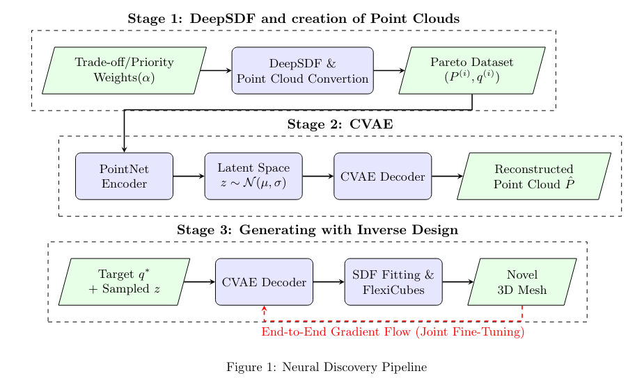
This pipeline is composed of 3 parts, as shown in Fig1.
This is, if you are a normal undergraduate student who has only taken Deep/Machine Learning, probably the hardest part of the project, to really grasp. To understand this part: the prerequisites such as the definition of Signed Distance Function, and DeepSDF mechanics will be explained here.
Definition 1. Let \( \Omega \subset \mathbb{R}^3 \) be a bounded open set (the shape interior) with boundary \( \partial\Omega \) (the surface). The signed distance function (SDF) of \( \Omega \) is:
$$ S(\mathbf{x}) = \begin{cases} -d(\mathbf{x}, \partial\Omega) & \mathbf{x} \in \Omega \\ 0 & \mathbf{x} \in \partial\Omega \\ +d(\mathbf{x}, \partial\Omega) & \mathbf{x} \notin \Omega \end{cases} $$where \( d(\mathbf{x}, \partial\Omega) = \inf_{\mathbf{y} \in \partial\Omega} \|\mathbf{x} - \mathbf{y}\|_2 \) is the unsigned distance to the surface.
Intuitively, it works like this: the function gets the point's location/coordinates, and outputs the distance between the point and the closest point on the shape. This output is positive when the point is outside the shape, 0 on the boundary of the shape, \( \partial\Omega \), and negative when the point is inside the shape (if inside, it will still look for the closest point on the boundary of the shape, now the output will just be negative).
The surface is recovered implicitly as the zero level set \( \partial\Omega = \{ \mathbf{x} \in \mathbb{R}^3 : S(\mathbf{x}) = 0 \} \). A key identity of true SDFs is the Eikonal equation:
$$ \|\nabla S(\mathbf{x})\|_2 = 1 \quad \text{almost everywhere in } \mathbb{R}^3 $$The unit outward normal to the surface at a point \( \mathbf{x} \in \partial\Omega \) is \( \mathbf{\hat{n}}(\mathbf{x}) = \nabla S(\mathbf{x}) \).
This is essential to the mechanics of the project, because if the object only learns where the surface is, the values away from the surface could be anything. The Eikonal equation forces the gradient magnitude to be exactly 1 everywhere.
For a NN, this is a cleaner way to represent a shape than a mesh of triangles, because every point in space has a defined value.
This paper from 2019 is the first to successfully use a Deep NN to represent an entire class of complex 3D shapes, with OR without using Signed Distance Functions, in a continuous and differentiable way.
It parameterises the SDF \( S \) as a neural network mapping:
$$ S_{\theta}(\mathbf{x}; \mathbf{z}) : \mathbb{R}^3 \times \mathbb{R}^{d_z} \to \mathbb{R} $$\( \theta \) represents the network weights, \( \mathbf{z} \in \mathbb{R}^{d_z} \) is a shape latent code. Each shape in the dataset is assigned its own unique latent \( \mathbf{z} \), which is optimised jointly with \( \theta \) during training through a process known as auto-decoding.
Why not ReLU? Because ReLU is not twice-differentiable. And certain properties such as surface area need this property. But we can get the SoftPlus function to be closer and closer to ReLU putting high values as \( \beta \).
To find the different shapes that make up the Pareto front, we cannot just maximize/minimize one objective. Would not make sense! For this there is a technique called weighted scalarisation. We assign a weight vector \( \alpha \) to our objectives, and minimize the combined loss:
$$ \mathcal{L}_{obj}(\theta, z, \alpha) = -\sum_{i=1}^{k} \alpha_i f_i(S_{\theta}(\cdot; z)) $$By sweeping through different values of \( \alpha \) (for example, putting 90% weight on volume and 10% on surface area, then 80/20, etc.), we can discover a diverse set of optimal shapes.
Normal geometric properties often require integrating non-differentiable functions over a space. Since I need a differentiable approximation, I can approximate these integrals using Monte Carlo sampling over a bounding box \(\mathcal{B}\) containing \(M\) sampled points \(\{x_m\}_{m=1}^M \sim \mathcal{U}(\mathcal{B})\). Mathematical properties like the following I had to search deeply.
Before the project, I did not know most of these terms, such as Hausdorff Measure, Normal Field, Divergence etc. so I feel the need to explain at least some of these mathematical terms.
Not everything is as mathematically smooth as volume or surface area. For properties that simply cannot be differentiated (like structural stability evaluated by a finite-element simulation), One can train a surrogate neural network to predict the objective straight from the shape's latent code. For shadow coverage and projected silhouettes, he/she can use Nvdiffrast, which makes rendering fully differentiable.
Once Stage 1 finished, I had a beautiful dataset of diverse, Pareto-optimal shapes. But Neural SDFs are continuous, making them tricky to feed directly into standard deep learning encoders. To bridge this gap, I discretised each shape by sampling a dense point cloud right near its zero level set.
From there, I trained a Conditional Variational Autoencoder (CVAE). If you have worked with generative models before, the setup will look familiar, but with a few geometric twists:
If an architect comes to me and says, "I need a shape with exactly 0.30 normalised volume and 0.70 surface area," here is how the pipeline delivers:
To measure success, I calculated the Property Satisfaction Error (PSE), which tells us exactly how far off our generated shape's properties are from the targets we asked for.
In Stage 1, the pipeline did a good job discovering the Pareto front, smoothly capturing the morphological transition from compact, volume-minimising spheres to faceted, low-surface-area shapes. When we got to the generative Inverse Design in Stage 3, shapes in the middle of our trade-off space achieved a very low median PSE (between 0.22 and 0.49).
However, the error spiked to around 0.78 for extreme edge cases (like demanding maximum volume but minimum surface area). This asymmetry mostly comes down to the small dataset (only 50 shapes means sparse coverage at the extremes) and a low Marching Cubes resolution introducing discretisation error. Both of these are straightforward to fix with more compute—by scaling up the dataset and resolution, this pipeline proves we can turn costly, discrete optimisations into an instant, queryable generative model for 3D engineering.